MissPath-FM

Flow Matching with Structured Priors for Partially Observed Time Series

When part of a sequence is already observed, the flow should not start from pure noise. MissPath-FM starts the transport near the observed signal and spends it on the entries that are actually missing.

NeurIPS 2026

Genpei Zhang

Department of Computer Sciences, University of Wisconsin–Madison

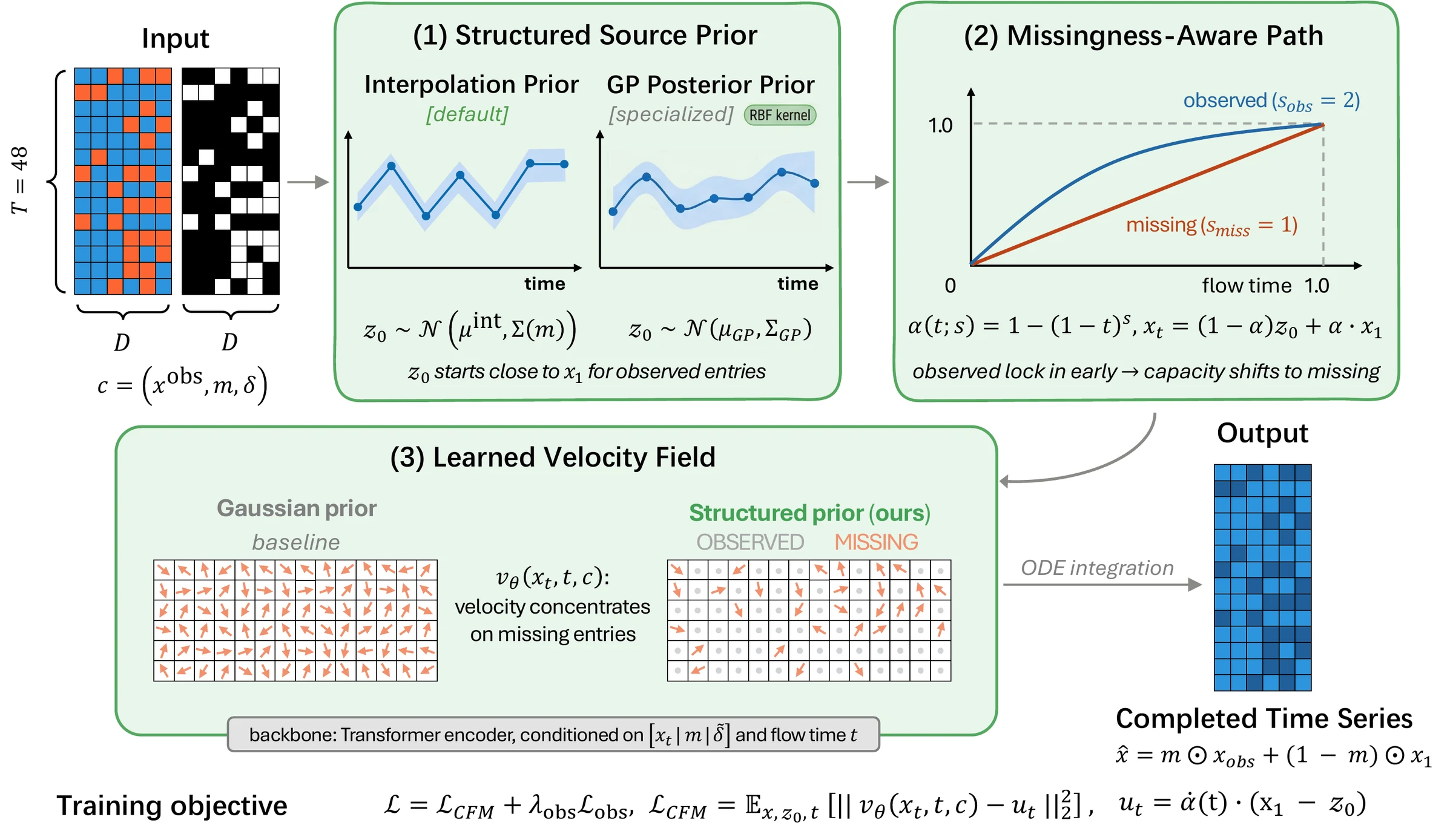
Overview of MissPath-FM: a structured source prior, a missingness-aware path, and a context-conditioned velocity field.
Overview of MissPath-FM. (1) A structured source prior initializes \(z_0\) close to the observed signal. (2) A missingness-aware path (\(s_{\mathrm{obs}} > s_{\mathrm{miss}}\)) locks in observed entries early. (3) A context-conditioned Transformer predicts the velocity; at inference, \(z_0\) is integrated with 20 Euler steps and observed entries are restored.

Abstract

A Gaussian source wastes the flow on what is already known.

Flow matching has emerged as a powerful alternative to diffusion models for generative modeling, but standard conditional flow matching is fundamentally misaligned with partially observed time series: starting from an uninformed Gaussian source forces the model to transport even already-observed entries from noise to the target, wasting capacity on trivially known regions.

We propose MissPath-FM, a partial-observation-aware flow matching framework that redesigns the source prior and probability path for incomplete time series. MissPath-FM employs structured source priors (interpolation priors and Gaussian process posterior priors) to initialize the flow close to the observed signal, paired with a missingness-aware smooth path that allocates transport asymmetrically between observed and missing regions.

We evaluate systematically across four datasets, four missingness mechanisms (MCAR, block, MNAR, irregular), two missing ratios, and three sequence lengths (\(T \in \{24, 48, 96\}\)), totaling 48 settings against eight baselines. MissPath-FM wins 29 of 32 settings at \(T{=}48\) and 45 of 48 overall (93.8%). Our ablations reveal a regime-dependent design hierarchy in which no single component suffices: under random missingness the source prior yields a large initial gain, but under structured block missingness it can fail entirely and the learned flow becomes indispensable; the missingness-aware path contributes a further 12%–26% across all regimes. Mechanistically, structured priors shorten observed-region transport by up to 15×, concentrating the velocity field on genuinely uncertain entries.
The bottleneck

Where does the transport go?

Under the linear path \(x_t = (1-t)\,z_0 + t\,x_1\), the expected transport cost splits by observation status. With a Gaussian source, every observed entry still has to be carried from noise to its known value.

Transport cost decomposition (Proposition 1)

\[\mathbb{E}\bigl[\|x_1 - z_0\|^2\bigr] = \mathcal{C}_{\mathrm{obs}} + \mathcal{C}_{\mathrm{miss}}, \qquad \mathcal{C}_{\mathrm{obs}} = \sum_{m_{\tau,d}=1} \mathbb{E}\bigl[(x_{1,\tau,d} - z_{0,\tau,d})^2\bigr]\]
Gaussian source

\(z_0 \sim \mathcal{N}(0, I)\)

For z-scored data each observed entry costs 2, so \(\mathcal{C}_{\mathrm{obs}} = 2\,n_{\mathrm{obs}}\): the cost grows with the number of entries the model already knows. At 50% missingness, about half of the network's capacity goes to them.

Interpolation source

\(z_0 = x_1 + \epsilon\) on observed entries

With \(\epsilon \sim \mathcal{N}(0, \sigma_{\mathrm{obs}}^2)\), \(\mathcal{C}_{\mathrm{obs}} = \sigma_{\mathrm{obs}}^2\, n_{\mathrm{obs}} \to 0\). The flow only has real work to do where values are missing.

Method

Three components, used together in every result

Structured source prior

Start from \(z_0 \sim \mathcal{N}(\mu^{\mathrm{int}}, \Sigma(m))\): piecewise-linear interpolation of the observations, with small noise \(\sigma_{\mathrm{obs}}\) on observed entries and larger \(\sigma_{\mathrm{miss}}\) on missing ones. A GP posterior prior is an optional alternative.

Missingness-aware path

Each entry moves at its own speed, \(\alpha_{\tau,d}(t) = 1-(1-t)^{s_{\tau,d}}\) with \(s_{\mathrm{obs}} > s_{\mathrm{miss}}\). Observed entries settle early, so later in the flow the velocity field effectively works only on the missing ones.

Context-conditioned velocity

A Transformer over time takes \([x_t \,\|\, m \,\|\, \tilde\delta]\) per step (values, mask, time since last observation) plus flow-time embeddings. Inference uses 20 Euler steps, then restores observed entries.

Path, target velocity and loss

\[x_{t,\tau,d} = \bigl(1 - \alpha_{\tau,d}(t)\bigr)\,z_{0,\tau,d} + \alpha_{\tau,d}(t)\,x_{1,\tau,d}, \qquad u_{t,\tau,d} = s_{\tau,d}\,(1-t)^{s_{\tau,d}-1}\,(x_{1,\tau,d} - z_{0,\tau,d})\]
\[\mathcal{L} = \mathbb{E}_{x,\, z_0,\, t}\bigl\| v_{\theta}(x_t, t, c) - u_t \bigr\|_2^2 + \lambda_{\mathrm{obs}}\,\mathcal{L}_{\mathrm{obs}}, \qquad \lambda_{\mathrm{obs}} = 0.1\]

The complete training step

# (i) Interpolation prior
mu    = interp_1d(x_obs, mask)             # piecewise linear in time
sigma = where(mask, 0.1, 1.0)              # sigma_obs << sigma_miss
z0    = mu + sigma * randn_like(mu)

# (ii) Missingness-aware path
s     = where(mask, 2.0, 1.0)              # s_obs = 2, s_miss = 1
alpha = 1 - (1 - t) ** s
x_t   = (1 - alpha) * z0 + alpha * x1
u_t   = s * (1 - t) ** (s - 1) * (x1 - z0)

# (iii) Loss: CFM on all entries + light observed-entry term
err   = (v_theta(x_t, t, ctx) - u_t) ** 2
loss  = err.mean() + 0.1 * (mask * err).sum() / mask.sum()

Results

Imputation, forecasting and generation

Four datasets (Synthetic, ETTm1, Electricity, PhysioNet 2012), four missingness mechanisms (MCAR, Block, MNAR, Irregular) at two ratios, against eight baselines under identical splits and masks.

45 / 48 Settings won overall (93.8%), across \(T \in \{24, 48, 96\}\)
29 / 32 Settings won at \(T{=}48\), average rank 1.16 among nine methods
6 / 6 Forecasting settings won at horizon \(h{=}24\), clean and corrupted histories
15× Shorter transport on observed entries with a structured prior

Imputation (MAE ↓, \(T{=}48\))

MechanismRateFlowTSCLWFTSFlowPSW-ISAITSBRITSCSDIGP-VAEOurs
MCAR30%0.3930.1900.1210.1440.0960.1030.1590.4540.075
MCAR50%0.4310.2240.1320.1620.1090.1220.2030.5830.085
Block30%0.3960.1970.2450.2650.1520.1600.2480.5110.106
Block50%0.4500.2490.2670.3200.1990.2380.3580.5720.145
MNAR30%0.4390.3660.1860.2430.1430.1860.2190.7460.117
MNAR50%0.4820.3820.2440.2850.2160.2690.2730.7930.158
Irregular30%0.4440.3820.1440.1880.1340.1410.2460.7350.101
Irregular50%0.4610.3270.1410.1880.1320.1450.5320.7310.101

Best in bold, second best underlined. The three losses: Electricity Block 30% and 50% (BRITS, SAITS) and PhysioNet MNAR 50% (SAITS, by 4%). PhysioNet keeps its natural sparsity (~19% observed) with an additional artificial hold-out.

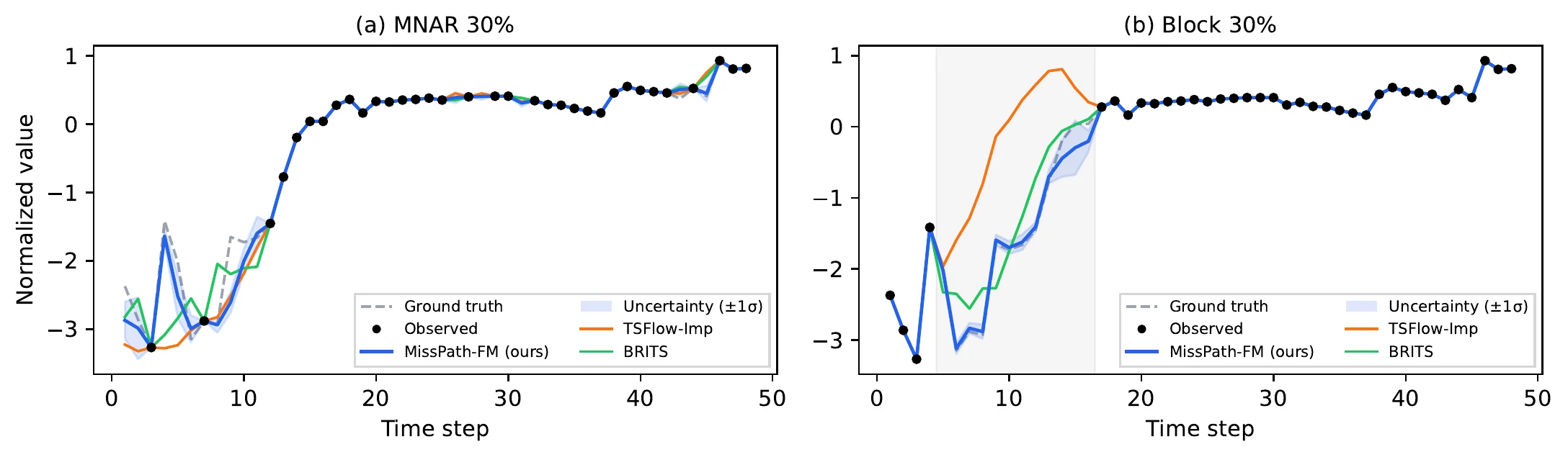
Qualitative imputation on ETTm1 under MNAR and Block missingness.
Qualitative imputation on ETTm1. (a) MNAR 30%: MissPath-FM recovers masked extreme values where baselines deviate. (b) Block 30%: within the contiguous gap (shaded), TSFlow diverges and BRITS flattens, while MissPath-FM tracks the ground truth with calibrated uncertainty.

What drives the gains? (incremental ablation, MAE ↓)

DatasetSetting(A) Gaussian + Flow(B) Interp. prior(C) GP prior(D) + Flow matching(E) + Context(F) + MA pathΔ flow
ETTm1MCAR 30%0.73870.10910.12140.09180.08560.0751−31%
Block 30%0.72480.21620.41500.13350.12530.1057−51%
SyntheticMCAR 30%0.81650.16140.10890.12080.11820.0981−10%
Block 30%0.80560.85740.63260.55780.49380.3737−41%
ElectricityMCAR 30%0.40280.18970.22300.12380.11370.0910−52%
Block 30%0.41420.84170.73950.27890.25030.2158−71%
PhysioNetArtificial 10%0.63550.36320.41190.33050.30570.2271−37%
Block 30%0.63070.37370.44040.34200.32480.2610−30%

Each column adds one component. Δ flow: gain of (F) over the best prior-only column.

No single component is enough. Under random missingness the prior gives the largest single gain (43%–85%). Under block missingness, interpolation alone can fail outright (Electricity: 0.842, worse than a Gaussian flow) because contiguous gaps leave no flanking observations, and the learned flow does the recovery. The missingness-aware path adds a further 12%–26% in every regime.

Beyond imputation

Forecasting, \(h{=}24\) (MAE ↓)

DatasetHistorySAITSBRITSCSDIGP-VAEFlowTSCLWFTSFlowOurs
ETTm1Clean0.4890.6920.7630.6940.7020.4830.3550.266
30% MCAR0.5280.6920.5930.7040.6790.4800.3650.264
SyntheticClean0.7910.7811.0840.7870.8500.8250.5660.511
30% MCAR0.8060.7781.0710.7940.8500.8370.5730.572
ElectricityClean1.0400.8730.8610.9370.9350.9470.2260.149
30% MCAR0.8710.8211.0560.9070.9180.9530.2370.153

Unconditional generation (all ↓)

SyntheticETTm1Electricity
MethodDisc.Pred.Spec.Disc.Pred.Spec.Disc.Pred.Spec.
CSDI0.5000.9251.5400.4740.7451.3130.5000.6311.294
GP-VAE0.5000.8091.6570.5000.8871.0620.4770.5811.341
FlowTS0.2750.2660.1260.1840.2140.0450.2500.2790.112
TSFlow0.5000.9291.5380.5000.9061.6990.5000.7341.655
Gauss.+Std0.3000.2400.1550.1980.2860.2560.1820.2010.113
MissPath-FM0.1690.2610.0920.0640.1860.0080.1550.1410.104

Disc.: discriminative score; Pred.: predictive score; Spec.: spectral distance.

Why it works

The velocity field moves to the missing entries

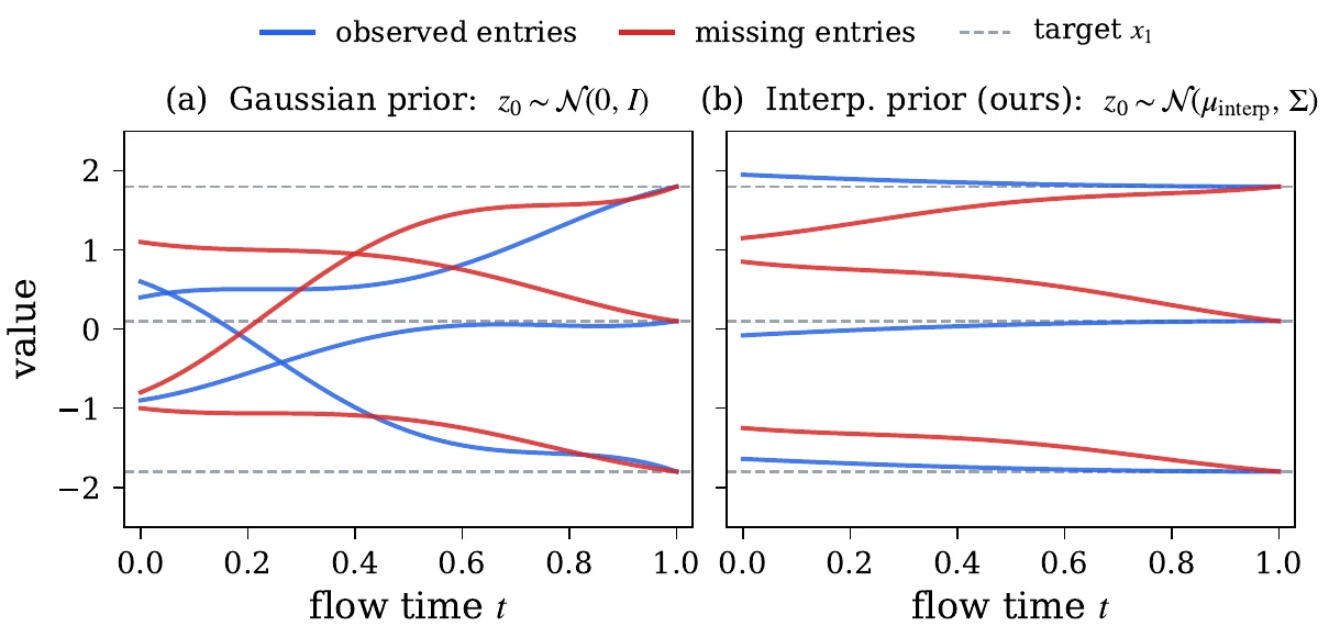
With a Gaussian prior, every entry travels a long way from noise. With a structured prior, observed entries barely move, and the miss-to-observed transport ratio rises from 1.1× to 19.2×.

Transport trajectories under a Gaussian prior and an interpolation prior.
Transport trajectories under a Gaussian prior (a) and an interpolation prior (b).

Trajectory length (Synthetic, Block 50%)

ConfigMAEℓ obsℓ missRatio
Gauss.+Std0.8820.7160.7571.1×
Interp+Std0.6510.0470.90619.2×
Interp+MA0.6340.0480.89518.9×
GP+Std0.5580.0430.55713.0×
GP+MA0.5340.0420.55213.1×

ℓ obs / ℓ miss: mean arc length on observed / missing entries. The GP prior also shortens missing-region transport by 39%.

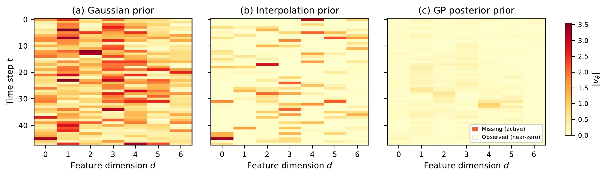
Velocity field magnitude at t = 0.5 under Gaussian, interpolation and GP posterior priors.
Velocity magnitude \(\|v_\theta\|\) at \(t{=}0.5\) (ETTm1, MCAR 30%). (a) Gaussian prior: velocity is spread across all entries. (b) Interpolation prior: observed entries are silenced and velocity concentrates on missing entries. (c) GP posterior prior: missing-entry velocity is reduced further, since the posterior mean starts closer to the target.

Citation

Cite MissPath-FM

If you find this work useful, please consider citing:

@inproceedings{zhang2026misspath,
  title     = {MissPath-FM: Flow Matching with Structured Priors for Partially Observed Time Series},
  author    = {Zhang, Genpei},
  booktitle = {Advances in Neural Information Processing Systems (NeurIPS)},
  year      = {2026}
}